Osmosis
The phenomenon of osmosis (from the Greek word for ‘push’) is the spontaneous passage of a pure solvent into a solution separated from it by a semipermeable mem brane, a membrane permeable to the solvent but not to the solute (Fig. 5.27). The osmotic pressure, Π, is the pressure that must be applied to the solution to stop the influx of solvent. Important examples of osmosis include transport of fluids through cell membranes, dialysis and osmometry, the determination of molar mass by the measurement of osmotic pressure. Osmometry is widely used to determine the molar masses of macromolecules. In the simple arrangement shown in Fig. 5.28, the opposing pressure arises from the head of solution that the osmosis itself produces. Equilibrium is reached when the hydrostatic pressure of the column of solution matches the osmotic pressure. The complicating feature of this arrangement is that the entry of solvent into the solution results in its dilution, and so it is more difficult to treat than the arrangement in Fig. 5.27, in which there is no flow and the concentrations remain unchanged. The thermodynamic treatment of osmosis depends on noting that, at equilibrium, the chemical potential of the solvent must be the same on each side of the membrane. The chemical potential of the solvent is lowered by the solute, but is restored to its ‘pure’ value by the application of pressure. As shown in the Justification below, this equality implies that for dilute solutions the osmotic pressure is given by the van ’t Hoff equation:
Π=[B]RT
where [B] = nB/V is the molar concentration of the solute.
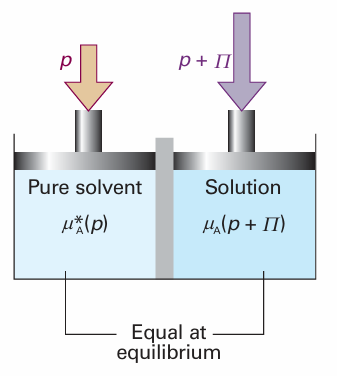
Fig. 5.27 The equilibrium involved in the calculation of osmotic pressure, Π, is between pure solvent A at a pressure p on one side of the semipermeable membrane and A as a component of the mixture on the other side of the membrane, where the pressure is p + Π.
Justification 5.3 The van ’t Hoff equation On the pure solvent side the chemical potential of the solvent, which is at a pressure p, is µA*(p). On the solution side, the chemical potential is lowered by the presence of the solute, which reduces the mole fraction of the solvent from 1 to xA. However, the chemical potential of A is raised on account of the greater pressure, p + Π, that the solution experiences. At equilibrium the chemical potential of A is the same in both compartments, and we can write
µA*(p) = µA (xA, p + Π)
The presence of solute is taken into account in the normal way:
µA (xA, p + Π) =µA*(p+Π) +RTlnxA
We saw in Section 3.9c (eqn 3.54) how to take the effect of pressure into account:
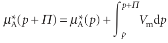
Where Vm is the molar volume of the pure solvent A. When these three equations are combined we get
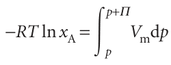
This expression enables us to calculate the additional pressure Π that must be applied to the solution to restore the chemical potential of the solvent to its ‘pure’ value and thus to restore equilibrium across the semipermeable membrane. For dilute solutions, ln xA may be replaced by ln (1 − xB) ≈−xB. We may also assume that the pressure range in the integration is so small that the molar volume of the solvent is a constant. That being so, Vm may be taken outside the integral, giving
RTxB=ΠVm
When the solution is dilute, xB ≈ nB/nA. Moreover, because nAVm = V, the total volume of the solvent, the equation simplifies to eqn 5.40.
Because the effect of osmotic pressure is so readily measurable and large, one of the most common applications of osmometry is to the measurement of molar masses of macromolecules, such as proteins and synthetic polymers. As these huge molecules dissolve to produce solutions that are far from ideal, it is assumed that the van ’t Hoff equation is only the first term of a virial-like expansion:4
Π=[J]RT{1+B[J]+· · · }
The additional terms take the nonideality into account; the empirical constant B is called the osmotic virial coefficient
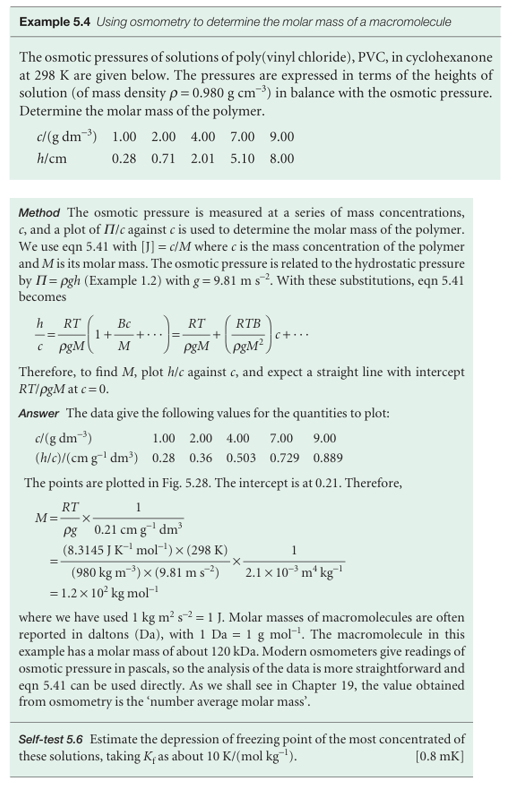
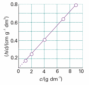
Fig. 5.28The plot involved in the determination of molar mass by osmometry. The molar mass is calculated from the intercept at c=0; in Chapter 19 we shall see that additional information comes from the slope.
Osmosis helps biological cells maintain their structure. Cell membranes are semiper meable and allow water, small molecules, and hydrated ions to pass, while blocking the passage of biopolymers synthesized inside the cell. The difference in concentrations of solutes inside and outside the cell gives rise to an osmotic pressure, and water passes into the more concentrated solution in the interior of the cell, carrying small nutrient molecules. The influx of water also keeps the cell swollen, whereas dehydration causes the cell to shrink. These effects are important in everyday medical practice. To maintain the integrity of blood cells, solutions that are injected into the bloodstream for blood transfusions and intravenous feeding must be isotonic with the blood, meaning that they must have the same osmotic pressure as blood. If the injected solution is too dilute, or hypotonic, the flow of solvent into the cells, required to equalize the osmotic pressure, causes the cells to burst and die by a process called haemolysis.If the solution is too concentrated, or hypertonic, equalization of the osmotic pressure requires flow of solvent out of the cells, which shrink and die.
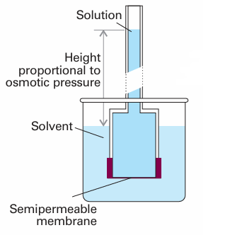
Fig. 5.29 In a simple version of the osmotic pressure experiment, A is at equilibrium on each side of the membrane when enough has passed into the solution to cause a hydrostatic pressure difference.
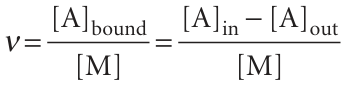
Osmosis also forms the basis of dialysis, a common technique for the removal of impurities from solutions of biological macromolecules and for the study of binding of small molecules to macromolecules, such as an inhibitor to an enzyme, an antibi otic to DNA, and any other instance of cooperation or inhibition by small molecules attaching to large ones. In a purification experiment, a solution of macromolecules containing impurities, such as ions or small molecules (including small proteins or nucleic acids), is placed in a bag made of a material that acts as a semipermeable membrane and the filled bag is immersed in a solvent. The membrane permits the passage of the small ions and molecules but not the larger macromolecules, so the former migrate through the membrane, leaving the macromolecules behind. In practice, purification of the sample requires several changes of solvent to coax most of the impurities out of the dialysis bag. In a binding experiment, a solution of macromolecules and smaller ions or molecules is placed in a dialysis bag, which is then immersed in a solvent. Suppose the molar concentration of the macromolecule M is [M] and the total concentration of the small molecule A in the bag is [A]in. This total concentration is the sum of the concentrations of free A and bound A, which we write [A]free and [A]bound, respectively. At equilibrium, the chemical potential of free A in the macromolecule solution is equal to the chemical potential of A in the solution on the other side of the membrane, where its concentration is [A]out. We shall see in Section 5.7 that the equality µA, free = µA, out implies that [A]free = [A]out, provided the activity coefficient of A is the same in both solutions. Therefore, by measuring the concentration of A in the ‘outside’ solution, we can find the concentration of unbound A in the macromolecule solution and, from the difference [A]in − [A]free, which is equal to [A]in − [A]out, the concentration of bound A. The average number of A molecules bound to M molecules, ν, is then the ratio
The bound and unbound A molecules are in equilibrium, M + A → MA, so their concentrations are related by an equilibrium constant K, where
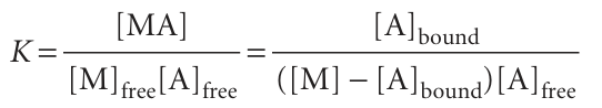
We have used [MA] = [A]bound and [M]free = [M] − [MA] = [M] − [A]bound. On division by [M], and replacement of [A]free by [A]out, the last expression becomes
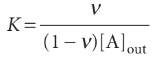
If there are N identical and independent binding sites on each macromolecule, each macromolecule behaves like N separate smaller macromolecules, with the same value of K for each site. The average number of A molecules per site is ν/N, so the last equation becomes
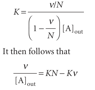
This expression is the Scatchard equation. It implies that a plot of ν/[A]out against v should be a straight line of slope −K and intercept KN at ν = 0 (see Fig. 5.30). From these two quantities, we can find the equilibrium constant for binding and the number of binding sites on each macromolecule. If a straight line is not obtained, we can conclude that the binding sites are not equivalent or independent.
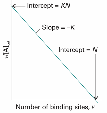
Fig. 5.30 A Scatchard plot of ν/[A]out against ν. The slope is –K and the intercept at ν = 0 is KN.
 الاكثر قراءة في مواضيع عامة في الكيمياء الفيزيائية
 اخر الاخبار
اخبار العتبة العباسية المقدسة


