
The depression of freezing point
 المؤلف:
Peter Atkins، Julio de Paula
المؤلف:
Peter Atkins، Julio de Paula
 المصدر:
ATKINS PHYSICAL CHEMISTRY
المصدر:
ATKINS PHYSICAL CHEMISTRY
 الجزء والصفحة:
ص152-153
الجزء والصفحة:
ص152-153
 2025-11-13
 75
75
The depression of freezing point
The heterogeneous equilibrium now of interest is between pure solid solvent A and the solution with solute present at a mole fraction xB (Fig. 5.24). At the freezing point, the chemical potentials of A in the two phases are equal:
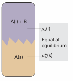
Fig. 5.24The heterogeneous equilibrium involved in the calculation of the lowering of freezing point is between A in the pure solid and A in the mixture, A being the solvent and B a solute that is insoluble in solid A.
µA*(s) = µA*(l) + RT ln xA
The only difference between this calculation and the last is the appearance of the solid’s chemical potential in place of the vapour’s. Therefore, we can write the result directly from eqn 5.33:
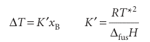
where ∆Tis the freezing point depression, T* − T, and ∆fusH is the enthalpy of fusion of the solvent. Larger depressions are observed in solvents with low enthalpies of fusion and high melting points. When the solution is dilute, the mole fraction is proportional to the molality of the solute, b, and it is common to write the last equation as
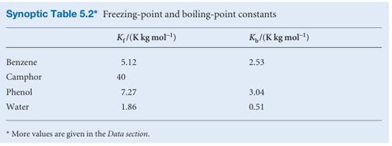
∆T=Kfb , where Kf is the empirical freezing-point constant (Table 5.2). Once the freezing point constant of a solvent is known, the depression of freezing point may be used to measure the molar mass of a solute in the method known as cryoscopy; however, the technique is of little more than historical interest.
 الاكثر قراءة في مواضيع عامة في الكيمياء الفيزيائية
 اخر الاخبار
اخبار العتبة العباسية المقدسة


