Binomial Distribution

The binomial distribution gives the discrete probability distribution  of obtaining exactly  successes out of  Bernoulli trials (where the result of each Bernoulli trial is true with probability  and false with probability ). The binomial distribution is therefore given by

			(1)
			(2)

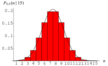
where  is a binomial coefficient. The above plot shows the distribution of  successes out of  trials with .

The binomial distribution is implemented in the Wolfram Language as BinomialDistribution[n, p].

The probability of obtaining more successes than the  observed in a binomial distribution is

(3)

where

(4)

 is the beta function, and  is the incomplete beta function.

The characteristic function for the binomial distribution is

(5)

(Papoulis 1984, p. 154). The moment-generating function  for the distribution is

			(6)
			(7)
			(8)
			(9)
			(10)
			(11)

The mean is

			(12)
			(13)
			(14)

The moments about 0 are

			(15)
			(16)
			(17)
			(18)

so the moments about the mean are

			(19)
			(20)
			(21)

The skewness and kurtosis excess are

			(22)
			(23)
			(24)
			(25)

The first cumulant is

(26)

and subsequent cumulants are given by the recurrence relation

(27)

The mean deviation is given by

(28)

For the special case , this is equal to

			(29)
			(30)

where  is a double factorial. For , 2, ..., the first few values are therefore 1/2, 1/2, 3/4, 3/4, 15/16, 15/16, ... (OEIS A086116 and A086117). The general case is given by

(31)

Steinhaus (1999, pp. 25-28) considers the expected number of squares  containing a given number of grains  on board of size  after random distribution of  of grains,

(32)

Taking  gives the results summarized in the following table.

0	23.3591
1	23.7299
2	11.8650
3	3.89221
4	0.942162
5	0.179459
6	0.0280109
7	0.0036840
8
9
10

An approximation to the binomial distribution for large  can be obtained by expanding about the value  where  is a maximum, i.e., where . Since the logarithm function is monotonic, we can instead choose to expand the logarithm. Let , then

(33)

where

(34)

But we are expanding about the maximum, so, by definition,

(35)

This also means that  is negative, so we can write . Now, taking the logarithm of (◇) gives

(36)

For large  and  we can use Stirling's approximation

(37)

so

			(38)
			(39)
			(40)
			(41)
			(42)

and

(43)

To find , set this expression to 0 and solve for ,

(44)

(45)

(46)

(47)

since . We can now find the terms in the expansion

			(48)
			(49)
			(50)
			(51)
			(52)
			(53)
			(54)
			(55)
			(56)
			(57)
			(58)
			(59)

Now, treating the distribution as continuous,

(60)

Since each term is of order  smaller than the previous, we can ignore terms higher than , so

(61)

The probability must be normalized, so

(62)

and

			(63)
			(64)

Defining ,

(65)

which is a normal distribution. The binomial distribution is therefore approximated by a normal distribution for any fixed  (even if  is small) as  is taken to infinity.

If  and  in such a way that , then the binomial distribution converges to the Poisson distribution with mean .

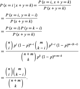
Let  and  be independent binomial random variables characterized by parameters  and . The conditional probability of  given that  is

(66)

Note that this is a hypergeometric distribution.

REFERENCES:

Beyer, W. H. CRC Standard Mathematical Tables, 28th ed. Boca Raton, FL: CRC Press, p. 531, 1987.

Papoulis, A. Probability, Random Variables, and Stochastic Processes, 2nd ed. New York: McGraw-Hill, pp. 102-103, 1984.

Press, W. H.; Flannery, B. P.; Teukolsky, S. A.; and Vetterling, W. T. "Incomplete Beta Function, Student's Distribution, F-Distribution, Cumulative Binomial Distribution." §6.2 in Numerical Recipes in FORTRAN: The Art of Scientific Computing, 2nd ed. Cambridge, England: Cambridge University Press, pp. 219-223, 1992.

Spiegel, M. R. Theory and Problems of Probability and Statistics. New York: McGraw-Hill, pp. 108-109, 1992.

Steinhaus, H. Mathematical Snapshots, 3rd ed. New York: Dover, 1999.