This was experimental mathematics par excellence, an approach to the subject in which mathematicians had their laboratory benches just like the physicists and chemists. They too could now do experiments. New vistas opened up – literally. It was a liberation from the arid climes of ‘definition, theorem, proof’, though a return to the rigours of rational argument would have to come albeit later.

The downside of this experimental approach was that the visual images preceded a theoretical underpinning. Experimentalists were navigating without a map. Although Mandelbrot coined the word ‘fractals’, what were they? Could there be a precise definition for them in the usual way of mathematics? In the beginning, Mandelbrot didn’t want to do this. He didn’t want to destroy the magic of the experience by honing a sharp definition which might be inadequate and limiting. He felt the notion of a fractal, ‘like a good wine – demanded a bit of aging before being “bottled”.’

The Mandelbrot set

Mandelbrot and his colleagues were not being particularly abstruse mathematicians. They were playing with the simplest of formulae. The whole idea is based on iteration – the practice of applying a formula time and time again. The formula which generated the Mandelbrot set was simply x² + c.

The first thing we do is choose a value of c. Let’s choose c = 0.5. Starting with x = 0 we substitute into the formula x² + 0.5. This first calculation gives 0.5 again. We now use this as x, substituting it into x² + 0.5 to give a second calculation: (0.5)² + 0.5 = 0.75. We keep going, and at the third stage this will be (0.75)² + 0.5 = 1.0625. All these calculations can be done on a handheld calculator. Carrying on we find that the answer gets bigger and bigger.

Let’s try another value of c, this time c = – 0.5. As before we start at x = 0 and substitute it into x² – 0.5 to give – 0.5. Carrying on we get – 0.25, but this time the values do not become bigger and bigger but, after some oscillations, settle down to a figure near – 0.3660. . .

So by choosing c = 0.5 the sequence starting at x = 0 zooms off to infinity, but by choosing c = – 0.5 we find that the sequence starting at x = 0 actually converges to a value near – 0.3660. The Mandelbrot set consists of all those values of c for which the sequence starting at x = 0 does not escape to infinity.

The Mandelbrot set

This is not the whole story because so far we have only considered the one-dimensional real numbers – giving a one-dimensional Mandelbrot set so we wouldn’t see much. What needs to be considered is the same formula z² + c but with z and c as two-dimensional complex numbers . This will give us a two-dimensional Mandelbrot set.

For some values of c in the Mandelbrot set, the sequence of zs may do all sorts of strange things like dance between a number of points but they will not escape to infinity. In the Mandelbrot set we see another key property of fractals, that of self-similarity. If you zoom into the set you will not be sure of the level of magnification because you will just see more Mandelbrot sets.

Before Mandelbrot

Like most things in mathematics, discoveries are rarely brand new. Looking into the history Mandelbrot found that mathematicians such as Henri Poincaré and Arthur Cayley had brief glimmerings of the idea a hundred years before him. Unfortunately they did not have the computing power to investigate matters further.

The shapes discovered by the first wave of fractal theorists included crinkly curves and the ‘monster curves’ that had previously been dismissed as pathological examples of curves. As they were so pathological they had been locked up in the mathematician’s cupboard and given little attention. What was wanted then were the more normal ‘smooth’ curves which could be dealt with by the differential calculus. With the popularity of fractals, other mathematicians whose work was resurrected were Gaston Julia and Pierre Fatou who worked on fractal-like structures in the complex plane in the years following the First World War. Their curves were not called fractals, of course, and they did not have the technological equipment to see their shapes.

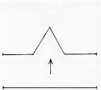
The generating element of the Koch snowflake

Other famous fractals

The famous Koch curve is named after the Swedish mathematician Niels Fabian Helge von Koch. The snowflake curve is practically the first fractal curve. It is generated from the side of the triangle treated as an element, splitting it into three parts each of length ⅓ and adding a triangle in the middle position.

The Koch snowflake

The curious property of the Koch curve is that it has a finite area, because it always stays within a circle, but at each stage of its generation its length increases. It is a curve which encloses a finite area but has an ‘infinite’ circumference!

Another famous fractal is named after the Polish mathematician Wacław Sierpinski. It is found by subtracting triangles from an equilateral triangle; and by continuing this process, we get the Sierpinski gasket.

The Sierpin ski gasket

Fractional dimension

The way Felix Hausdorff looked at dimension was innovative. It has to do with scale. If a line is scaled up by a factor of 3 it is 3 times longer than it was previously. Since this 3 = 3¹ a line is said to have dimension 1. If a solid square is scaled up by a factor of 3 its area is 9 times its previous value or 3² and so the dimension is 2. If a cube is scaled up by this factor its volume is 27 or 3³ times its previous value, so its dimension is 3. These values of the Hausdorff dimension all coincide with our expectations for a line, square, or cube.

If the basic unit of the Koch curve is scaled up by 3, it becomes 4 times longer than it was before. Following the scheme described, the Hausdorff dimension is the value of D for which 4 = 3^D. An alternative calculation is that

which means that D for the Koch curve is approximately 1.262. With fractals it is frequently the case that the Hausdorff dimension is greater than the ordinary dimension, which is 1 in the case of Koch curve.

The Hausdorff dimension informed Mandelbrot’s definition of a fractal – a set of points whose value of D is not a whole number. Fractional dimension became the key property of fractals.

The applications of fractals

The potential for the applications of fractals is wide. Fractals could well be the mathematical medium which models such natural objects as plant growth, or cloud formation.

Fractals have already been applied to the growth of marine organisms such as corals and sponges. The spread of modern cities has been shown to have a similarity with fractal growth. In medicine they have found application in the modelling of brain activity. And the fractal nature of movements of stocks and shares and the foreign exchange markets has also been investigated. Mandelbrot’s work opened up a new vista and there is much still to be discovered.

the condensed idea

Shapes with fractional dimension

مواضيع ذات صلة

π

Zero

Triangles

Topology

The travelling salesperson

The Riemann hypothesis

The parallel postulate

The normal curve

The four-colour problem

The diet problem

The birthday problem

Squares and square roots