تاريخ الرياضيات

الاعداد و نظريتها
تاريخ التحليل
تار يخ الجبر
الهندسة و التبلوجي
الرياضيات في الحضارات المختلفة
العربية
اليونانية
البابلية
الصينية
المايا
المصرية
الهندية
الرياضيات المتقطعة
المنطق
اسس الرياضيات
فلسفة الرياضيات
مواضيع عامة في المنطق
الجبر
الجبر الخطي
الجبر المجرد
الجبر البولياني
مواضيع عامة في الجبر
الضبابية
نظرية المجموعات
نظرية الزمر
نظرية الحلقات والحقول
نظرية الاعداد
نظرية الفئات
حساب المتجهات
المتتاليات-المتسلسلات
المصفوفات و نظريتها
المثلثات
الهندسة
الهندسة المستوية
الهندسة غير المستوية
مواضيع عامة في الهندسة
التفاضل و التكامل
المعادلات التفاضلية و التكاملية
معادلات تفاضلية
معادلات تكاملية
مواضيع عامة في المعادلات
التحليل
التحليل العددي
التحليل العقدي
التحليل الدالي
مواضيع عامة في التحليل
التحليل الحقيقي
التبلوجيا
نظرية الالعاب
الاحتمالات و الاحصاء
نظرية التحكم
بحوث العمليات
نظرية الكم
الشفرات
الرياضيات التطبيقية
نظريات ومبرهنات
علماء الرياضيات
500AD
500-1499
1000to1499
1500to1599
1600to1649
1650to1699
1700to1749
1750to1779
1780to1799
1800to1819
1820to1829
1830to1839
1840to1849
1850to1859
1860to1864
1865to1869
1870to1874
1875to1879
1880to1884
1885to1889
1890to1894
1895to1899
1900to1904
1905to1909
1910to1914
1915to1919
1920to1924
1925to1929
1930to1939
1940to the present
علماء الرياضيات
الرياضيات في العلوم الاخرى
بحوث و اطاريح جامعية
هل تعلم
طرائق التدريس
الرياضيات العامة
نظرية البيان

Distributions
 المؤلف:
Tony Crilly
المؤلف:
Tony Crilly
 المصدر:
50 mathematical ideas you really need to know
المصدر:
50 mathematical ideas you really need to know
 الجزء والصفحة:
197-201
الجزء والصفحة:
197-201
 21-2-2016
 1888
1888


+
-
20
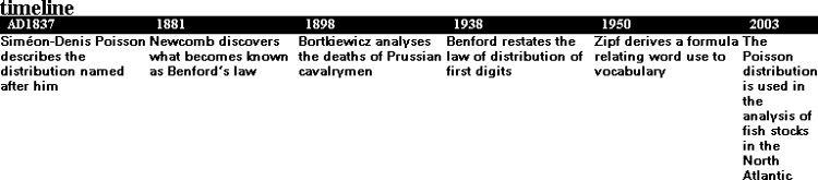
Ladislaus J. Bortkiewicz was fascinated by mortality tables. Not for him a gloomy topic, they were a field of enduring scientific enquiry. He famously counted the number of cavalrymen in the Prussian army that had been killed by horse-kicks. Then there was Frank Benford, an electrical engineer who counted the first digits of different types of numerical data to see how many were ones, twos and so on. And George Kingsley Zipf, who taught German at Harvard, had an interest in philology and analysed the occurrences of words in pieces of text.
All these examples involve measuring the probabilities of events. What are the probabilities of x cavalrymen in a year receiving a lethal kick from a horse? Listing the probabilities for each value of x is called a distribution of probabilities, or for short, a probability distribution. It is also a discrete distribution because the values of x only take isolated values – there are gaps between the values of interest. You can have three or four Prussian cavalrymen struck down by a lethal horse-kick but not 3½. As we’ll see, in the case of the Benford distribution we are only interested in the appearance of digits 1, 2, 3, . . . and, for the Zipf distribution, you may have the word ‘it’ ranked eighth in the list of leading words, but not at position, say 8.23.
Life and death in the Prussian army
Bortkiewicz collected records for ten corps over a 20 year period giving him data for 200 corps-years. He looked at the number of deaths (this was what mathematicians call the variable) and the number of corps-years when this number of deaths occurred. For example, there were 109 corps-years when no deaths occurred, while in one corps-year, there were four deaths. At the barracks, Corp C (say) in one particular year experienced four deaths.
How is the number of deaths distributed? Collecting this information is one side of the statistician’s job – being out in the field recording results. Bortkiewicz obtained the following data:

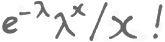
The Poisson formula
Thankfully, being killed by a horse-kick is a rare event. The most suitable theoretical technique for modelling how often rare events occur is to use something called the Poisson distribution. With this technique, could Bortkiewicz have predicted the results without visiting the stables? The theoretical Poisson distribution says that the probability that the number of deaths (which we’ll call X) has the value x is given by the Poisson formula, where e is the special number discussed earlier that’s associated with growth and the exclamation mark means the factorial, the number multiplied by all the other whole numbers between it and 1 . The Greek letter lambda, written λ, is the average number of deaths. We need to find this average over our 200 corps-years so we multiply 0 deaths by 109 corps-years (giving 0), 1 death by 65 corps-years (giving 65), 2 deaths by 22 corps-years (giving 44), 3 deaths by 3 corps-years (giving 9) and 4 deaths by 1 corps-year (giving 4) and then we add all of these together (giving 122) and divide by 200. So our average number of deaths per corps-year is 122/200 = 0.61.
The theoretical probabilities (which we’ll call p) can be found by substituting the values r = 0, 1, 2, 3 and 4 into the Poisson formula. The results are:
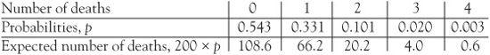
It looks as though the theoretical distribution is a good fit for the experimental data gathered by Bortkiewicz.
First numbers
If we analyse the last digits of telephone numbers in a column of the telephone directory we would expect to find 0, 1, 2, . . . , 9 to be uniformly distributed. They appear at random and any number has an equal chance of turning up. In 1938 the electrical engineer Frank Benford found that this was not true for the first digits of some sets of data. In fact he rediscovered a law first observed by the astronomer Simon Newcomb in 1881.
Yesterday I conducted a little experiment. I looked through the foreign currency exchange data in a national newspaper. There were exchange rates like 2.119 to mean you will need (US dollar) $2.119 to buy £1 sterling. Likewise, you will need (Euro) ∊1.59 to buy £1 sterling and (Hong Kong dollar) HK $15.390 to buy £1. Reviewing the results of the data and recording the number of appearances by first digit, gave the following table:
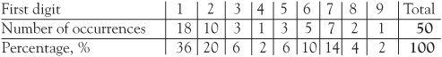
These results support Benford’s law, which says that for some classes of data, the number 1 appears as the first digit in about 30% of the data, the number 2 in 18% of the data and so on. It is certainly not the uniform distribution that occurs in the last digit of the telephone numbers.
It is not obvious why so many data sets do follow Benford’s law. In the 19th century when Simon Newcomb observed it in the use of mathematical tables he could hardly have guessed it would be so widespread.
Instances where Benford’s distribution can be detected include scores in sporting events, stock market data, house numbers, populations of countries, and the lengths of rivers. The measurement units are unimportant – it does not matter if the lengths of rivers are measured in metres or miles. Benford’s law has practical applications. Once it was recognized that accounting information followed this law, it became easier to detect false information and uncover fraud.
Words
One of G.K. Zipf’s wide interests was the unusual practice of counting words. It turns out that the ten most popular words appearing in the English language are the tiny words ranked as shown:
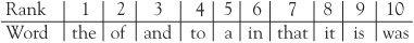
This was found by taking a large sample across a wide range of written work and just counting words. The most common word was given rank 1, the next rank 2, and so on. There might be small differences in the popularity stakes if a range of texts were analysed, but it will not vary much.
It is not surprising that ‘the’ is the most common, and ‘of’ is second. The list continues and you might want to know that ‘among’ is in 500th position and ‘neck’ is ranked 1000. We shall only consider the top ten words. If you pick up a text at random and count these words you will get more or less the same words in rank order. The surprising fact is that the ranks have a bearing on the actual number of appearances of the words in a text. The word ‘the’ will occur twice as often as ‘of’ and three times more frequently than ‘and’, and so on. The actual number is given by a well-known formula. This is an experimental law and was discovered by Zipf from data. The theoretical Zipf’s law says that the percentage of occurrences of the word ranked r is given by

where the number k depends only on the size of the author’s vocabulary. If an author had command of all the words in the English language, of which there are around a million by some estimates, the value of k would be about 0.0694. In the formula for Zipf’s law the word ‘the’ would then account for about 6.94% of all words in a text. In the same way ‘of’ would account for half of this, or about 3.47% of the words. An essay of 3000 words by such a talented author would therefore contain 208 appearances of ‘the’ and 104 appearances of the word ‘of’.
For writers with only 20,000 words at their command, the value of k rises to 0.0954, so there would be 286 appearances of ‘the’ and 143 appearances of the word ‘of’. The smaller the vocabulary, the more often you will see ‘the’ appearing.
Crystal ball gazing
Whether Poisson, Benford or Zipf, all these distributions allow us to make predictions. We may not be able to predict a dead cert but knowing how the probabilities distribute themselves is much better than taking a shot in the dark. Add to these three, other distributions like the binomial, the negative binomial, the geometric, the hypergeometric, and many more, the statistician has an effective array of tools for analysing a vast range of human activity.
the condensed idea
Predicting how many
 الاكثر قراءة في هل تعلم
 اخر الاخبار
اخبار العتبة العباسية المقدسة

الآخبار الصحية


 قسم الشؤون الفكرية يصدر كتاباً يوثق تاريخ السدانة في العتبة العباسية المقدسة
 "المهمة".. إصدار قصصي يوثّق القصص الفائزة في مسابقة فتوى الدفاع المقدسة للقصة القصيرة
 (نوافذ).. إصدار أدبي يوثق القصص الفائزة في مسابقة الإمام العسكري (عليه السلام)