1.1 Slope of a Straight Line

All students will be familiar with the equation for a straight line

  (1.1)

where c is the intercept on the y axis and m is the slope of the line. To prove to ourselves that m really is the slope, we need a good definition of slope. Let's define

  (1.2)

where Δy is the difference between final and initial values y_f and y_i.  The graph of y(x) = 2x+1 is plotted and the slope has been determined by measuring Δy and Δx. Rather than always having to verify the slope graphically, let's do it analytically for all lines. Take x_i = x as the initial x value and x_f = x +Δx as the final value. Obviously x_f - x_i = Δx. The initial value of y is

 (1.3)

and the final value is

 (1.4)

Thus Δy = y_f -y_i = m(x +Δx)+ c-mx-c = mΔx. Therefore the slope becomes

 (1.5)

which is a proof that y = mx + c has a slope of m. From above we can re-write our formula (1.2) using y_f = y(x + Δx) and y_i = y(x), so that

  (1.6)

1.2 Slope of a Curve

A straight line always has constant slope m. That's why it's called straight. The parabola y(x) = x² + 1 is plotted. In fact the concept of the slope of a parabola doesn't make any sense because the parabola continuously curves. However we might think about little pieces of the parabola. If you look at any tiny little piece it looks straight. These tiny little pieces are all tiny little line segments, each with their own slope. Notice that the slope of the tiny little line segments keeps changing. At x = 0 the slope is 0 (the tiny little line is flat) whereas around     x = 1 the slope is larger. One of the most important ideas in calculus is the concept of the derivative, which is nothing more than

Derivative = Slope of tiny little line segment.

we got the slope from Δy and Δx on the large triangle in the top right hand corner. But we would get the same answer if we had used the tiny triangles in the bottom left hand corner. What characterizes these tiny triangles is that Δx and Δy are both tiny (but their ratio,  always). Another way of saying that Δx is tiny is to say

That is the limit as Δx goes to zero is another way of saying Δx is tiny.

Examples

1)

2)

3)

4)

5)

For a curve like the parabola we can't draw a big triangle, because the hypotenuse would be curved. But we can get the slope at a point by drawing a tiny triangle at that point. Thus let's define the

So it's the same definition as before in (1.6) except is an instruction to use a tiny triangle. Now from (1.6) and the derivative is given a fancy new symbol  so that

 (1.7)

The symbol dy simply means

That is, usually Δy can be big or small. If we are talking about a tiny Δy we write dy instead. Similarly for Δx.

Example Calculate the derivative of the straight line y(x) = 3x

Solution

Thus the derivative is the slope.

Example Calculate the derivative of the straight line y(x) = 4

Solution

The line y(x) = 4 has 0 slope and therefore 0 derivative. The derivative was defined to give us the slope of a curve at a point. The two examples above show that it also works for a straight line (A straight line is a special case of a curve). Now do some examples for real curves.

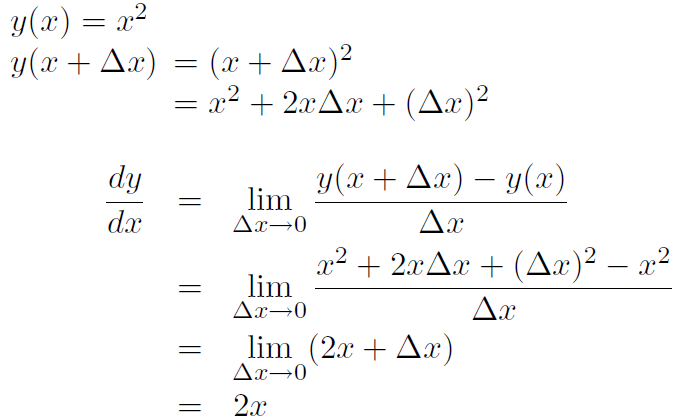
Example Calculate the derivative of the parabola y(x) = x²

Solution

Example Calculate the slope of the parabola y(x) = x² at the points x = -2, x = 0, x = 3.

Solution We already have . Thus

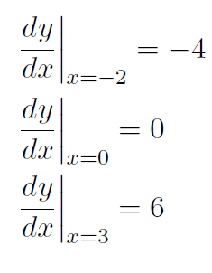
which shows how the slope of a tiny little line segment varies as we move along the parabola.

Example Calculate the slope of the curve y(x) = x² + 1 at the points x = -2, x = 0, x = 3

Solution

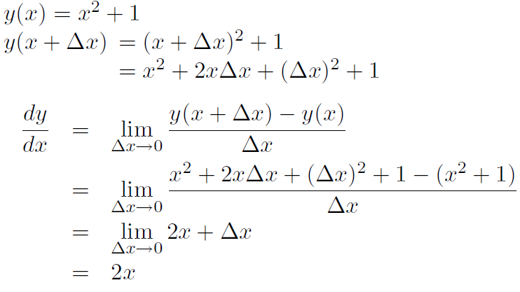
Thus the slopes are the same as in the previous example.

1.3 Some Common Derivatives

In a previous example we saw that the derivative of y(x) = 4 was , which make sense because a graph of y(x) = 4 reveals that the slope is always 0. This is true for any constant c. Thus

 (1.8)

We also saw in a previous example that . In general we have

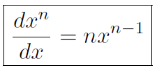 (1.9)

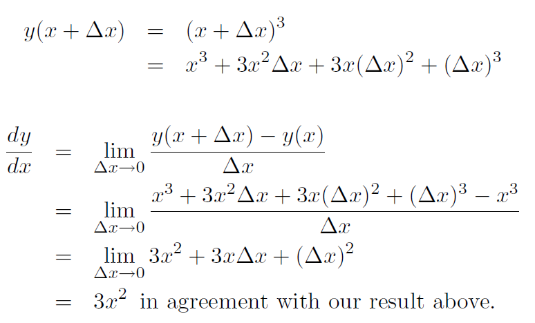
This is a very important result. We have already verified it for n = 2. Let's verify it for n = 3.

Example Check that (1.9) is correct for n = 3.

Solution Formula (1.9) gives

We wish to verify this. Take y(x) = x³.

A list of very useful results for derivatives is given below. You will prove most of these results in your calculus course. I will just make some comments about them.

Multiplicative constant rule

1. The derivative of a constant times a function equals the constant times the derivative of the function:

Addition rule

2. The derivative of a sum of functions equals the sum of the derivatives of the functions:

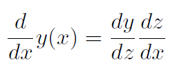
Chain rule

3. If y is a function of x and x is in turn a function of t, the derivative of y with respect to t equals the product of the derivative of y with respect to z and the derivative of z with respect to x:

Derivative of a product

4. The derivative of a product of functions y(x) z(x) equals the first function times the derivative of the second plus the second function times the derivative of the first:

Reciprocal derivative

5. The derivative of y with respect to x is the reciprocal of the derivative of x with respect to y, assuming that neither derivative is zero:

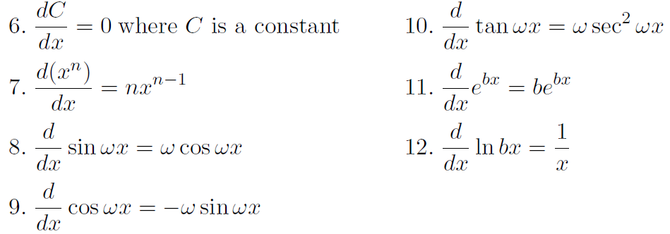
Derivatives of particular functions

Multiplicative constant rule Example

This just means, for example, that

Addition rule Example

Take for example y(x) = x and z(x) = x². This rule just means

Chain Rule  

(A rough ''proof" of this is to just note that the dz cancels in the numerator and denominator.) The use of the chain rule is best seen in the following example, where y is not given as a function of x.

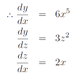
Example Verify the chain rule for y = z³ and z = x².

Solution We have y(z) = z³ and z(x) = x². Thus y(x) = x⁶.

Now   = (3z²)(2x) = (3x⁴)(2x) = 6x⁵. Thus we see that

Product Rule

The use of this arises when multiplying two functions together as illustrated in the next example.

Example If y(x) = x³ and z(x) = x², verify the product rule.

Solution

Now let's show that the product rule gives the same answer.

in agreement with our answer above.

1.4 Extremum Value of a Function

A final important use of the derivative is that it can be used to tell us when a function attains a maximum or minimum value. This occurs when the derivative or slope of the function is zero.

Example What are the (x, y) coordinates of the place where the parabola y(x) = x² + 3 has its minimum value?

Solution The minimum value occurs where the slope is 0. Thus

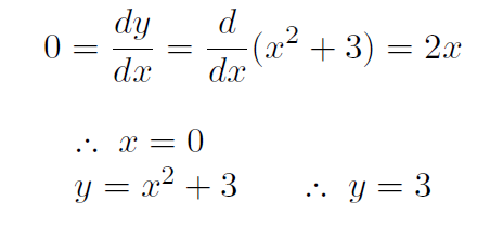
Thus the minimum is at (x, y) = (0, 3). You can verify this by plotting a graph.