
تاريخ الرياضيات

الاعداد و نظريتها

تاريخ التحليل

تار يخ الجبر

الهندسة و التبلوجي


الرياضيات في الحضارات المختلفة

العربية

اليونانية

البابلية

الصينية

المايا

المصرية

الهندية


الرياضيات المتقطعة

المنطق

اسس الرياضيات

فلسفة الرياضيات

مواضيع عامة في المنطق


الجبر

الجبر الخطي

الجبر المجرد

الجبر البولياني

مواضيع عامة في الجبر

الضبابية

نظرية المجموعات

نظرية الزمر

نظرية الحلقات والحقول

نظرية الاعداد

نظرية الفئات

حساب المتجهات

المتتاليات-المتسلسلات

المصفوفات و نظريتها

المثلثات


الهندسة

الهندسة المستوية

الهندسة غير المستوية

مواضيع عامة في الهندسة

التفاضل و التكامل


المعادلات التفاضلية و التكاملية

معادلات تفاضلية

معادلات تكاملية

مواضيع عامة في المعادلات


التحليل

التحليل العددي

التحليل العقدي

التحليل الدالي

مواضيع عامة في التحليل

التحليل الحقيقي

التبلوجيا

نظرية الالعاب

الاحتمالات و الاحصاء

نظرية التحكم

بحوث العمليات

نظرية الكم

الشفرات

الرياضيات التطبيقية

نظريات ومبرهنات


علماء الرياضيات

500AD

500-1499

1000to1499

1500to1599

1600to1649

1650to1699

1700to1749

1750to1779

1780to1799

1800to1819

1820to1829

1830to1839

1840to1849

1850to1859

1860to1864

1865to1869

1870to1874

1875to1879

1880to1884

1885to1889

1890to1894

1895to1899

1900to1904

1905to1909

1910to1914

1915to1919

1920to1924

1925to1929

1930to1939

1940to the present

علماء الرياضيات

الرياضيات في العلوم الاخرى

بحوث و اطاريح جامعية

هل تعلم

طرائق التدريس

الرياضيات العامة

نظرية البيان
INTRODUCTION-EXAMPLES
المؤلف:
Lawrence C. Evans
المصدر:
An Introduction to Mathematical Optimal Control Theory
الجزء والصفحة:
5-10
2-10-2016
1289
EXAMPLE 1: CONTROL OF PRODUCTION AND CONSUMPTION.
Suppose we own, say, a factory whose output we can control. Let us begin to construct a mathematical model by setting x(t) = amount of output produced at time t ≥ 0.
We suppose that we consume some fraction of our output at each time, and likewise can reinvest the remaining fraction. Let us denote
α(t) = fraction of output reinvested at time t ≥ 0.
This will be our control, and is subject to the obvious constraint that
0 ≤ α(t) ≤ 1 for each time t ≥ 0.
Given such a control, the corresponding dynamics are provided by the ODE

the constant k > 0 modelling the growth rate of our reinvestment. Let us take as a payoff functional

The meaning is that we want to maximize our total consumption of the output, our consumption at a given time t being (1−α(t))x(t). This model fits into our general framework for n = m = 1, once we put
A = [0, 1], f(x, a) = kax, r(x, a) = (1 − a)x, g ≡ 0.

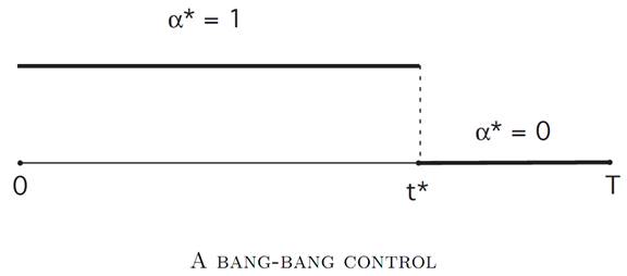
As we will see later , an optimal control α∗(.) is given by

for an appropriate switching time 0 ≤ t∗ ≤ T. In other words, we should reinvest all the output (and therefore consume nothing) up until time t∗, and afterwards, we should consume everything (and therefore reinvest nothing). The switchover time t∗ will have to be determined. We call α∗(.) a bang–bang control.
EXAMPLE 2: REPRODUCTIVE STATEGIES IN SOCIAL INSECTS
The next example is from (CONTROLLABILITY, BANG-BANG PRINCIPLE) of the book Caste and Ecology in Social Insects, by G. Oster and E. O. Wilson [O-W]. We attempt to model how social insects, say a population of bees, determine the makeup of their society.
Let us write T for the length of the season, and introduce the variables
w(t) = number of workers at time t
q(t) = number of queens
α(t) = fraction of colony effort devoted to increasing work force
The control α is constrained by our requiring that
0 ≤ α(t) ≤ 1.
We continue to model by introducing dynamics for the numbers of workers and the number of queens. The worker population evolves according to

Here μ is a given constant (a death rate), b is another constant, and s(t) is the known rate at which each worker contributes to the bee economy.
We suppose also that the population of queens changes according to

for constants ν and c.
Our goal, or rather the bees’, is to maximize the number of queens at time T:
P[α(.)] = q(T).
So in terms of our general notation, we have x(t) = (w(t), q(t))T and x0 = (w0, q0)T .
We are taking the running payoff to be r ≡ 0, and the terminal payoff g(w, q) = q.
The answer will again turn out to be a bang–bang control, as we will explain later.
EXAMPLE 3: A PENDULUM.
We look next at a hanging pendulum, for which
θ(t) = angle at time t.
If there is no external force, then we have the equation of motion

the solution of which is a damped oscillation, provided λ > 0.
Now let α(.) denote an applied torque, subject to the physical constraint that
|α| ≤ 1.
Our dynamics now become

Define

Then we can write the evolution as the system

We introduce as well

for

We want to maximize P[.], meaning that we want to minimize the time it takes to bring the pendulum to rest.
Observe that this problem does not quite fall within the general framework described in 1.1, since the terminal time is not fixed, but rather depends upon the
control. This is called a fixed endpoint, free time problem.
EXAMPLE 4: A MOON LANDER
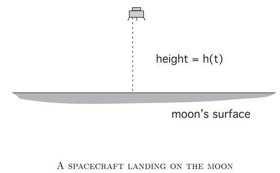
This model asks us to bring a spacecraft to a soft landing on the lunar surface, using the least amount of fuel.
We introduce the notation
h(t) = height at time t
v(t) = velocity = h˙ (t)
m(t) = mass of spacecraft (changing as fuel is burned)
α(t) = thrust at time t
We assume that
0 ≤ α(t) ≤ 1,
and Newton’s law tells us that

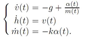
the right hand side being the difference of the gravitational force and the thrust of the rocket. This system is modeled by the ODE


We summarize these equations in the form

We want to minimize the amount of fuel used up, that is, to maximize the amount remaining once we have landed. Thus
P[α(.)] = m(τ ),
where
τ denotes the first time that h(τ ) = v(τ ) = 0.
This is a variable endpoint problem, since the final time is not given in advance.
We have also the extra constraints
h(t) ≥ 0, m(t) ≥ 0.
EXAMPLE 5: ROCKET RAILROAD CAR.
Imagine a railroad car powered by rocket engines on each side. We introduce the variables
q(t) = position at time t
v(t) = q˙ (t) = velocity at time t
α(t) = thrust from rockets,
where
−1 ≤ α(t) ≤ 1,

the sign depending upon which engine is firing.
We want to figure out how to fire the rockets, so as to arrive at the origin 0 with zero velocity in a minimum amount of time. Assuming the car has mass m, the law of motion is

We rewrite by setting x(t) = (q(t), v(t))T . Then

Since our goal is to steer to the origin (0, 0) in minimum time, we take

for
τ = first time that q(τ ) = v(τ ) = 0.
References
[B-CD] M. Bardi and I. Capuzzo-Dolcetta, Optimal Control and Viscosity Solutions of Hamilton-Jacobi-Bellman Equations, Birkhauser, 1997.
[B-J] N. Barron and R. Jensen, The Pontryagin maximum principle from dynamic programming and viscosity solutions to first-order partial differential equations, Transactions AMS 298 (1986), 635–641.
[C1] F. Clarke, Optimization and Nonsmooth Analysis, Wiley-Interscience, 1983.
[C2] F. Clarke, Methods of Dynamic and Nonsmooth Optimization, CBMS-NSF Regional Conference Series in Applied Mathematics, SIAM, 1989.
[Cr] B. D. Craven, Control and Optimization, Chapman & Hall, 1995.
[E] L. C. Evans, An Introduction to Stochastic Differential Equations, lecture notes avail-able at http://math.berkeley.edu/˜ evans/SDE.course.pdf.
[F-R] W. Fleming and R. Rishel, Deterministic and Stochastic Optimal Control, Springer, 1975.
[F-S] W. Fleming and M. Soner, Controlled Markov Processes and Viscosity Solutions, Springer, 1993.
[H] L. Hocking, Optimal Control: An Introduction to the Theory with Applications, OxfordUniversity Press, 1991.
[I] R. Isaacs, Differential Games: A mathematical theory with applications to warfare and pursuit, control and optimization, Wiley, 1965 (reprinted by Dover in 1999).
[K] G. Knowles, An Introduction to Applied Optimal Control, Academic Press, 1981.
[Kr] N. V. Krylov, Controlled Diffusion Processes, Springer, 1980.
[L-M] E. B. Lee and L. Markus, Foundations of Optimal Control Theory, Wiley, 1967.
[L] J. Lewin, Differential Games: Theory and methods for solving game problems with singular surfaces, Springer, 1994.
[M-S] J. Macki and A. Strauss, Introduction to Optimal Control Theory, Springer, 1982.
[O] B. K. Oksendal, Stochastic Differential Equations: An Introduction with Applications, 4th ed., Springer, 1995.
[O-W] G. Oster and E. O. Wilson, Caste and Ecology in Social Insects, Princeton UniversityPress.
[P-B-G-M] L. S. Pontryagin, V. G. Boltyanski, R. S. Gamkrelidze and E. F. Mishchenko, The Mathematical Theory of Optimal Processes, Interscience, 1962.
[T] William J. Terrell, Some fundamental control theory I: Controllability, observability, and duality, American Math Monthly 106 (1999), 705–719.
 الاكثر قراءة في نظرية التحكم
 اخر الاخبار
اخبار العتبة العباسية المقدسة

الآخبار الصحية


 قسم الشؤون الفكرية يصدر كتاباً يوثق تاريخ السدانة في العتبة العباسية المقدسة
 "المهمة".. إصدار قصصي يوثّق القصص الفائزة في مسابقة فتوى الدفاع المقدسة للقصة القصيرة
 (نوافذ).. إصدار أدبي يوثق القصص الفائزة في مسابقة الإمام العسكري (عليه السلام)


