Green's functions

Earlier on in this lecture course we had to solve Poisson's equation

 (1.1)

where v(r) is denoted the source function. The potential u(r) satisfies the boundary condition

 (1.2)

provided that the source function is reasonably localized. The solutions to Poisson's equation are superposable (because the equation is linear). This property is exploited in the Green's function method of solving this equation. The Green's function G(r, rʹ) is the potential, which satisfies the appropriate boundary conditions, generated by a unit amplitude point source located at rʹ. Thus,

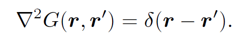 (1.3)

Any source function v(r) can be represented as a weighted sum of point sources

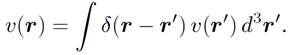 (1.4)

It follows from super posability that the potential generated by the source v(r) can be written as the weighted sum of point source driven potentials (i.e., Green's functions)

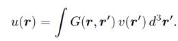 (1.5)

We found earlier that the Green's function for Poisson's equation is

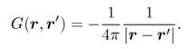 (1.6)

It follows that the general solution to Eq. (1.1) is written

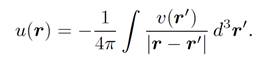 (1.7)

Note that the point source driven potential (1.6) is perfectly sensible. It is spherically symmetric about the source, and falls off smoothly with increasing distance from the source. We now need to solve the wave equation

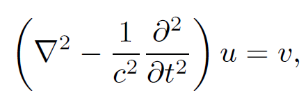 (1.8)

where v(r, t) is a time varying source function. The potential u(r, t) satisfies the boundary conditions

 (1.9)

The solutions to Eq. (1.8) are superposable (since the equation is linear), so a Green's function method of solution is again appropriate. The Green's function G(r, rʹ, t, tʹ) is the potential generated by a point impulse located at position rʹ and applied at time tʹ. Thus,

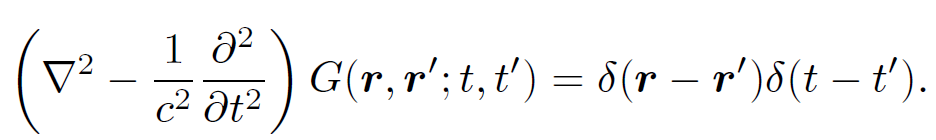 (1.10)

Of course, the Green's function must satisfy the correct boundary conditions. A general source v(r, t) can be built up from a weighted sum of point impulses

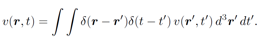 (1.11)

It follows that the potential generated by v(r, t) can be written as the weighted sum of point impulse driven potentials

 (1.12)

So, how do we find the Green's function? Consider

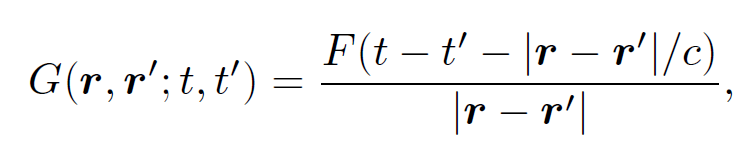 (1.13)

where F(ϕ) is a general scalar function. Let us try to prove the following theorem:

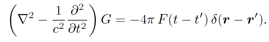 (1.14)

At a general point, r ≠ rʹ, the above expression reduces to

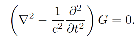 (1.15)

So, we basically have to show that G is a valid solution of the free space wave equation. We can easily show that

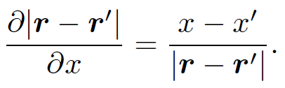 (1.16)

It follows by simple differentiation that

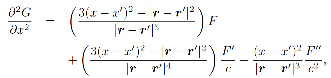 (1.17)

where Fʹ(ϕ) = dF(ϕ)=dϕ. We can derive analogous equations for ∂²G/∂y² and ∂²G/∂z². Thus,

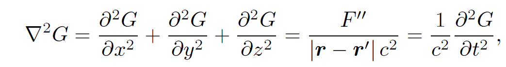 (1.18)

giving

 (1.19)

which is the desired result. Consider, now, the region around r = rʹ. It is clear from Eq. (1.17) that the dominant term on the left-hand side as |r - rʹ| → 0 is the first one, which is essentially F∂²(|r - rʹ|^-1)=∂x². It is also clear that (1/c²)(∂²G/∂t²) is negligible compared to this term. Thus, as |r - rʹ| → 0 we find that

 (1.20)

However, according to Eqs. (1.3) and (1.6)

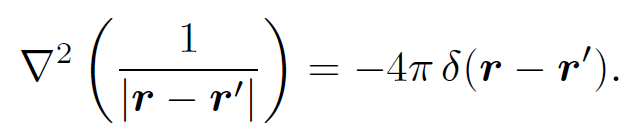 (1.21)

We conclude that

 (1.22)

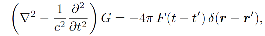
which is the desired result. Let us now make the special choice

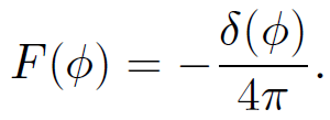 (1.23)

It follows from Eq. (1.22) that

 (1.24)

Thus,

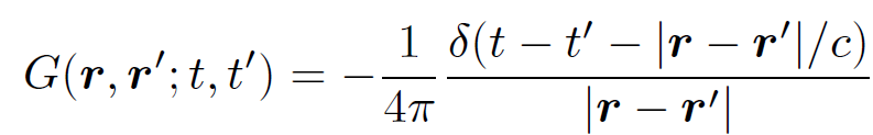 (1.25)

is the Green's function for the driven wave equation (1.8). The time dependent Green's function (1.25) is the same as the steady state Green's function (1.6), apart from the delta function appearing in the former. What does this delta function do? Well, consider an observer at point r. Because of the delta function our observer only measures a non-zero potential at one particular time

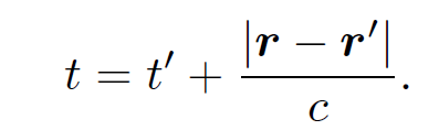 (1.26)

It is clear that this is the time the impulse was applied at position rʹ (i.e., tʹ) plus the time taken for a light signal to travel between points rʹ and r. At time t > tʹ the locus of all points at which the potential is non-zero is

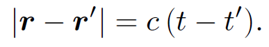 (1.27)

In other words, it is a sphere centred on rʹ whose radius is the distance traveled by light in the time interval since the impulse was applied at position rʹ. Thus, the Green's function (1.25) describes a spherical wave which emanates from position rʹ at time tʹ and propagates at the speed of light. The amplitude of the wave is inversely proportional to the distance from the source.

مواضيع ذات صلة

Thermal conductivity

Molecular diffusion

Ionic conductivity

The drift speed

Electrical transients

الشرر المقدس

الحقول الكهربية والشرر

الخلق غير المرئي

عجائب الكهرباء

مصادر الطاقة الكهربائية

التيارات الكهربائية التي تجري إلى الابد

النقل الكهربائي وقانون أوم