Gauss' law

Consider a single charge located at the origin. The electric field generated by such a charge is given by

 Suppose that we surround the charge by a concentric spherical surface S of radius r. The flux of the electric field through this surface is given by

 (1.1)

since the normal to the surface is always parallel to the local electric field. However, we also know from Gauss' theorem that

 (1.2)

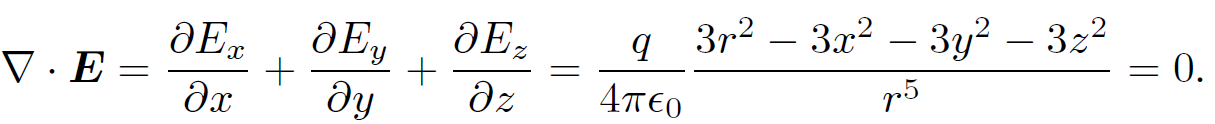
where V is the volume enclosed by surface S. Let us evaluate ∇. E directly. In Cartesian coordinates the field is written

 (1.3)

where r² = x² + y² + z². So,

 (1.4)

Here, use has been made of

 (1.5)

Formulae analogous to Eq. (1.4) can be obtained for ∂E_y/∂y and ∂E_z/∂z. The divergence of the field is given by

 (1.6)

This is a puzzling result! We have from Eqs. (1.1) and (1.2) that

 (1.7)

and yet we have just proved that ∇.E = 0. This paradox can be resolved after a close examination of Eq. (1.6). At the origin (r = 0) we find that ∇ . E = 0/0, which means that ∇ . E can take any value at this point. Thus, Eqs. (1.6) and (1.7) can be reconciled if ∇ . E is some sort of ''spike" function; i.e., it is zero everywhere except arbitrarily close to the origin, where it becomes very large. This must occur in such a manner that the volume integral over the ''spike" is finite. Let us examine how we might construct a one-dimensional ''spike" function. Consider the ''box-car" function

 (1.8)

It is clear that that

 (1.9)

Now consider the function

 (1.10)

This is zero everywhere except arbitrarily close to x = 0. According to Eq. (1.9), it also possess a finite integral;

 (1.11)

Thus, δ(x) has all of the required properties of a ''spike" function. The one-dimensional ''spike" function δ(x) is called the ''Dirac delta-function" after the Cambridge physicist Paul Dirac who invented it in 1927 while investigating quantum mechanics. The delta-function is an example of what mathematicians call a ''generalized function"; it is not well-defined at x = 0, but its integral is never- theless well-defined. Consider the integral

 (1.12)

where f(x) is a function which is well-behaved in the vicinity of x = 0. Since the delta-function is zero everywhere apart from very close to x = 0, it is clear that

 (1.13)

where use has been made of Eq. (1.11). The above equation, which is valid for any well-behaved function f(x), is effectively the definition of a delta-function. A simple change of variables allows us to define δ(x - x₀), which is a ''spike" function centred on x = x₀. Equation (1.13) gives

 (1.14)

We actually want a three-dimensional ''spike" function; i.e., a function which is zero everywhere apart from close to the origin, and whose volume integral is unity. If we denote this function by δ(r) then it is easily seen that the three-dimensional delta-function is the product of three one-dimensional delta- functions:

 (1.15)

This function is clearly zero everywhere except the origin. But is its volume integral unity? Let us integrate over a cube of dimensions 2a which is centred on the origin and aligned along the Cartesian axes. This volume integral is obviously separable, so that

 (1.16)

The integral can be turned into an integral over all space by taking the limit a → ∞. However, we know that for one-dimensional delta-functions , so it follows from the above equation that

 (1.17)

which is the desired result. A simple generalization of previous arguments yields

 (1.18)

where f(r) is any well-behaved scalar field. Finally, we can change variables and write

 (1.19)

which is a three-dimensional ''spike" function centred on r = rʹ. It is easily demonstrated that

 (1.20)

Up to now we have only considered volume integrals taken over all space. However, it should be obvious that the above result also holds for integrals over any finite volume V which contains the point r = rʹ. Likewise, the integral is zero if V does not contain r = rʹ. Let us now return to the problem in hand. The electric field generated by a charge q located at the origin has ∇ . E = 0 everywhere apart from the origin, and also satisfies

 (1.21)

for a spherical volume V centered on the origin. These two facts imply that

 (1.22)

where use has been made of Eq. (1.17). At this stage, you are probably not all that impressed with vector field theory. After all we have just spent an inordinately long time proving something using vector field theory which we previously proved in one line using conventional analysis! Let me now demonstrate the power of vector field theory. Consider, again, a charge q at the origin surrounded by a spherical surface S which is centered on the origin. Suppose that we now displace the surface S, so that it is no longer centered on the origin. What is the flux of the electric field out of S? This is no longer a simple problem for conventional analysis because the normal to the surface is not parallel to the local electric field. However, using vector field theory this problem is no more difficult than the previous one. We have

 (1.23)

from Gauss' theorem, plus Eq. (1.22). From these, it is clear that the flux of E out of S is q/ for a spherical surface displaced from the origin. However, the flux becomes zero when the displacement is sufficiently large that the origin is

no longer enclosed by the sphere. It is possible to prove this from conventional analysis, but it is not easy! Suppose that the surface S is not spherical but is instead highly distorted. What now is the flux of E out of S? This is a virtually impossible problem in conventional analysis, but it is easy using vector field theory. Gauss' theorem and Eq. (1.22) tell us that the flux is q/₀ provided that the surface contains the origin, and that the flux is zero otherwise. This result is independent of the shape of S.

Consider N charges qi located at ri. A simple generalization of Eq. (1.17) gives

 (1.24)

Thus, Gauss' theorem (1.23) implies that

 (1.25)

where Q is the total charge enclosed by the surface S. This result is called Gauss' law and does not depend on the shape of the surface. Suppose, finally, that instead of having a set of discrete charges we have a continuous charge distribution described by a charge density ρ(r). The charge contained in a small rectangular volume of dimensions dx, dy, and dz, located at position r is Q = ρ(r) dx dy dz. However, if we integrate ∇. E over this volume element we obtain

 (1.26)

where use has been made of Eq. (1.25). Here, the volume element is assumed to be sufficiently small that ∇. E does not vary significantly across it. Thus, we obtain

 (1.27)

This is the first of four field equations, called Maxwell's equations, which together form a complete description of electromagnetism. Of course, our derivation of Eq. (1.27) is only valid for electric fields generated by stationary charge distributions. In principle, additional terms might be required to describe fields generated by moving charge distributions. However, it turns out that this is not the case and that Eq. (1.27) is universally valid. Equation (1.27) is a differential equation describing the electric field generated by a set of charges. We already know the solution to this equation when the charges are stationary;

 (1.28)

Equations (1.27) and (1.28) can be reconciled provided

 (1.29)

It follows that

 (1.30)

which is the desired result. The most general form of Gauss' law, Eq. (1.25), is obtained by integrating Eq. (1.27) over a volume V surrounded by a surface S and making use of Gauss' theorem:

 (1.31)

مواضيع ذات صلة

Thermal conductivity

Molecular diffusion

Ionic conductivity

The drift speed

Electrical transients

الشرر المقدس

الحقول الكهربية والشرر

الخلق غير المرئي

عجائب الكهرباء

مصادر الطاقة الكهربائية

التيارات الكهربائية التي تجري إلى الابد

النقل الكهربائي وقانون أوم