The electric scalar potential

Suppose that r = (x, y, z) and rʹ = (xʹ, yʹ, zʹ) in Cartesian coordinates. The x component of (r - rʹ)/|r - rʹ|³ is written

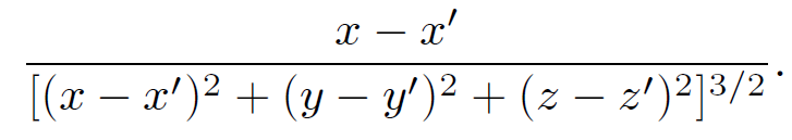 (1.1)

However, it is easily demonstrated that

 (1.2)

Since there is nothing special about the x-axis we can write

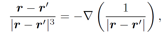 (1.3)

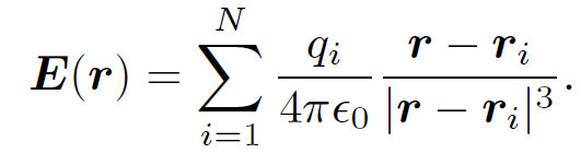
where ∇ ≡ (∂/∂x; ∂/∂y; ∂/∂z) is a differential operator which involves the components of r but not those of rʹ. That

 (1.4)

where

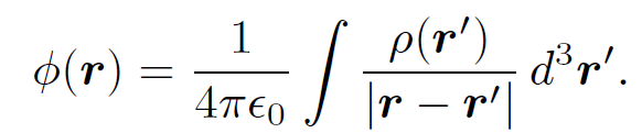 (1.5)

Thus, the electric field generated by a collection of fixed charges can be written as the gradient of a scalar potential, and this potential can be expressed as a simple volume integral involving the charge distribution. The scalar potential generated by a charge q located at the origin is

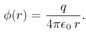 (1.6)

According to above as

the scalar potential generated by a set of N discrete charges q_i, located at r_i, is

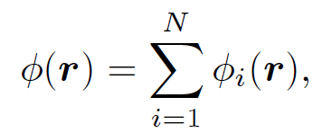 (1.7)

where

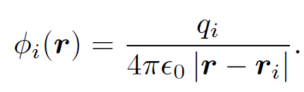 (1.8)

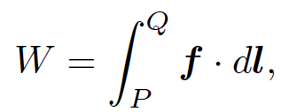
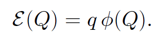
Thus, the scalar potential is just the sum of the potentials generated by each of the charges taken in isolation. Suppose that a particle of charge q is taken along some path from point P to point Q. The net work done on the particle by electrical forces is

 (1.9)

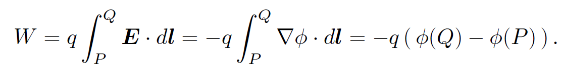
where f is the electrical force and dl is a line element along the path. We obtain

 (1.10)

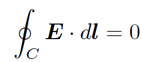
Thus, the work done on the particle is simply minus its charge times the difference in electric potential between the end point and the beginning point. This quantity is clearly independent of the path taken from P to Q. So, an electric field generated by stationary charges is an example of a conservative field. In fact, this result follows immediately from vector field theory once we are told, in Eq. (1.4), that the electric field is the gradient of a scalar potential. The work done on the particle when it is taken around a closed path is zero, so

 (1.11)

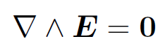
for any closed loop C. This implies from Stokes' theorem that

 (1.12)

for any electric field generated by stationary charges. Equation (1.12) also follows directly from Eq. (1.4), since ∇ ˄ ∇ϕ = 0 for any scalar potential ϕ. The SI unit of electric potential is the volt, which is equivalent to a joule per coulomb. Thus, according to Eq. (1.10) the electrical work done on a particle when it is taken between two points is the product of its charge and the voltage difference between the points. We are familiar with the idea that a particle moving in a gravitational field possesses potential energy as well as kinetic energy. If the particle moves from point P to a lower point Q then the gravitational field does work on the particle causing its kinetic energy to increase. The increase in kinetic energy of the particle is balanced by an equal decrease in its potential energy so that the overall energy of the particle is a conserved quantity. Therefore, the work done on the particle as it moves from P to Q is minus the difference in its gravitational potential energy between points Q and P. Of course, it only makes sense to talk about gravitational potential energy because the gravitational field is conservative. Thus, the work done in taking a particle between two points is path independent and, therefore, well defined. This means that the difference in potential energy of the particle between the beginning and end points is also well defined. We have already seen that an electric field generated by stationary charges is a conservative field. In follows that we can define an electrical potential energy of a particle moving in such a field. By analogy with gravitational fields, the work done in taking a particle from point P to point Q is equal to minus the difference in potential energy of the particle between points Q and P. It follows from Eq. (1.10) that the potential energy of the particle at a general point Q, relative to some reference point P, is given by

 (1.13)

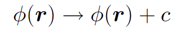
Free particles try to move down gradients of potential energy in order to attain a minimum potential energy state. Thus, free particles in the Earth's gravitational field tend to fall downwards. Likewise, positive charges moving in an electric field tend to migrate towards regions with the most negative voltage and vice versa for negative charges. The scalar electric potential is undefined to an additive constant. So, the transformation

 (1.14)

leaves the electric field unchanged according to Eq. (1.4). The potential can be fixed unambiguously by specifying its value at a single point. The usual convention is to say that the potential is zero at infinity. This convention is implicit in Eq. (1.5), where it can be seen that ϕ → 0 as |r| → ∞ provided that the total charge ∫ ρ(rʹ) d³rʹ is finite.

مواضيع ذات صلة

Thermal conductivity

Molecular diffusion

Ionic conductivity

The drift speed

Electrical transients

الشرر المقدس

الحقول الكهربية والشرر

الخلق غير المرئي

عجائب الكهرباء

مصادر الطاقة الكهربائية

التيارات الكهربائية التي تجري إلى الابد

النقل الكهربائي وقانون أوم