Suppose the University wants to estimate satisfaction with a new course. They might choose a sample of 200 students and ask them whether they enjoyed the course. Say 46 of the students say they enjoyed it. These 46 students are 23% of the sample,  so we call 23% the sample proportion. The percentage of students who actually enjoyed the course is called the population proportion. Assuming the sample of 200 students was unbiased, the University’s best guess for the population proportion is 23%.

In this example, a number of people were asked to give an opinion. This is called an opinion poll. These are very often used to evaluate products, test public opinion of political candidates, and so on. A random sample is chosen and the sample proportion is found. This is the best guess as to the population proportion, and of course it is important to know how confident one can be of the result.

Assume we are discussing a proportion (such as “proportion voting for a candidate” or “proportion voting yes”) and estimating it by sampling. We shall write p for the population proportion, and ˆp (“p-hat”) for the corresponding sample proportion. It will be convenient always to write these as percentages.

If you count 1 for each “yes” and 0 for each “no,” p is the population mean and pˆis the sample mean. So pˆ has approximately a normal distribution, and ˆp is the best estimator of p.

If the sample size is n, then ˆp has mean p and standard deviation σp, where it can be shown that approximately

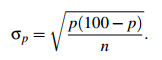
(This approximate standard deviation is quite accurate for large n, for example if n is at least 1,000.)

The best estimate for this standard deviation is

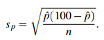
So we assume that there is a 95% chance that p lies in the range from pˆ− 2s_p to pˆ +2sp.

Sample Problem 1.1 In a survey of 1600 voters, 960 say they intend to vote Democrat at the next election. What is the 95% confidence interval for the percentage of voters who will vote Democrat?

Solution. In this case n = 1600 and

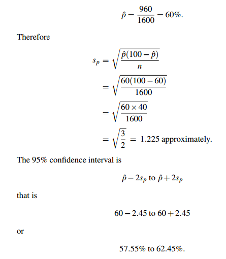
(This is often written as 60±2.45%.)

If there had been only 100 people in the survey, sp would have been 4.9, and the 95% confidence interval would have been

                            50.2% to 69.8%.

—not nearly so accurate.

There is another way of thinking about the 95% confidence level, which may give you a better idea of what it means. Suppose you went through the process of finding the 95% confidence interval for every possible sample. Then in 95% of cases the true population parameter value (mean, proportion, or whatever) would lie in the interval.

مواضيع ذات صلة

Trial

Sampling

Sample Proportion

Sample

Poisson Trials

Experiment

Wiener Numbers

Time Series Analysis

Spencer,s Formula

Redundancy

Predictability

Moving Average