The following example illustrates an application of spanning trees.

Sample Problem 1.1 Suppose an oil field contains five oil wells w₁, w₂, w₃, w₄, w₅, and a depot d. It is required to build pipelines so that oil can be pumped from the wells to the depot. Oil can be relayed from one well to another, at very small cost. All the workers involved will be company employees, so the only real expense is building the pipelines. Figure 1.1a shows which pipelines are feasible to build, represented as a graph in the obvious way, with the cost (in hundreds of thousands of dollars) shown. (If there is no edge between two vertices, the cost of a direct join between them would be very high.) Which pipelines should be built?

Solution. Your first impulse might be to connect d to each well directly, as shown in Fig. 8.1b. This would cost $2,600,000. However, the cheapest solution is shown in Fig. 1.1c, and costs $1,600,000.

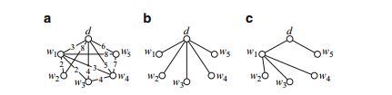
                Fig. 1.1 An oil pipeline problem

Once the pipelines in case (c) have been built, there is no reason to build a direct connection from d to w₃. Any oil being sent from w3 to the depot can be relayed through w₁. Similarly, there would be no point in building a pipeline joining w₃ to w₄. The conditions of the problem imply that the graph does not need to contain any cycle. However, it must be connected. So the solution is to find a spanning tree.

Moreover, the company would prefer the cheapest possible spanning tree. So we are interested in a minimum-cost spanning tree.

We shall look at an algorithm first described by Joseph Kruskal in 1956; not surprisingly, it is called Kruskal’s algorithm. Here is how it works.

First of all, select the cheapest edge in the graph. Then select the next cheapest edge. At every subsequent stage, go through the edges and delete any edge that would complete a cycle when combined with some of the edges already chosen.

Continue in this fashion. If, at any stage, there are two cheapest edges available,  choose either one. The end result will be a spanning tree, and it can be shown that this method always gives a cheapest possible tree.

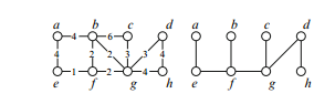
Fig. 1.2 Finding a minimum-cost spanning tree

As an example, consider the graph on the left of Fig. 1.2. The cheapest edge is e f , cost 1. The next cheapest cost is 2, and we can choose any one of f g, b f or bg.  Say we select f g. For the third edge we can choose either b f or bg; whichever one is chosen, the other will no longer be available, because we need to avoid the cycle bfg. We shall select f g. There are two edges of cost 3, namely cg and dg. We shall use cg. Then dg is still available, so we choose it for the fifth edge. At cost 4, there are four choices: dg, gh, ab, and ae. Say we select dh; then gh must be eliminated.

Finally, we choose ae, and ab is no longer available. The tree is complete, and is shown in the right-hand diagram.

Sample Problem 1.2 Suppose you are in the process of using Kruskal’s algorithm to find a minimum-cost spanning tree in the graph shown. Heavy line edges are those selected so far. Which edge would you choose next?

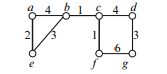
Solution. The available edges are ab, cd, and f g. But ab is disqualified because it would complete the cycle abe. Of the two remaining, cd is cheaper, so it is chosen.

                  Fig. 1.3 An example of Kruskal’s algorithm

Sample Problem 1.3 Find a minimal spanning tree in the graph G shown in Fig. 1.3a.

Solution. We start by listing the edges in order of cost: de, cost 1; be, cost 2; c f ,  cost 3; ab, cost 4; ad, cost 5; bc and e f , each cost 6. The first edge chosen is de.

مواضيع ذات صلة

Minimum Spanning Tree

Maximum Leaf Number

Lobster Graph

Labeled Tree

Internal Path Length

Red-Black Tree

Pseudotree

Pseudoforest

Prüfer Code

Planted Tree

Planted Planar Tree

Graph Strength