To solve the system of differential equations

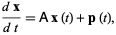(1)

where  is a matrix and  and  are vectors, first consider the homogeneous case with . The solutions to

(2)

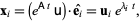
are given by

(3)

But, by the eigen decomposition theorem, the matrix exponential can be written as

(4)

where the eigenvector matrix is

(5)

and the eigenvalue matrix is

(6)

Now consider

			(7)
			(8)
			(9)

The individual solutions are then

(10)

so the homogeneous solution is

(11)

where the s are arbitrary constants.

The general procedure is therefore

1. Find the eigenvalues of the matrix  (, ..., ) by solving the characteristic equation.

2. Determine the corresponding eigenvectors , ..., .

3. Compute

(12)

for , ..., . Then the vectors  which are real are solutions to the homogeneous equation. If  is a  matrix, the complexvectors  correspond to real solutions to the homogeneous equation given by  and .

4. If the equation is nonhomogeneous, find the particular solution given by

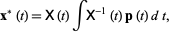(13)

where the matrix  is defined by

(14)

If the equation is homogeneous so that , then look for a solution of the form

(15)

This leads to an equation

(16)

so  is an eigenvector and  an eigenvalue.

5. The general solution is